3 Forensic parameters
In this chapter, we’ll show how to compute forensic parameters using STRAF, and provide details on how they are computed and should be interpreted. We’ll introduce a few equations, but please do not be afraid! The goal of this chapter is to translate each of them into plain English.
3.1 How to compute forensic parameters in STRAF
Once your data has been uploaded, you can go to the Forensic parameters tab and check the Compute forensics statistics box. The computation will be performed and a table containing the values per locus will be displayed. The computation is done per population and overall, a drop-down menu is present to select the population.
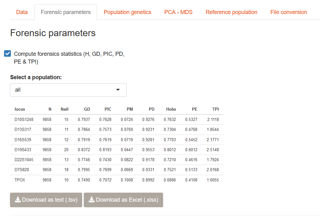
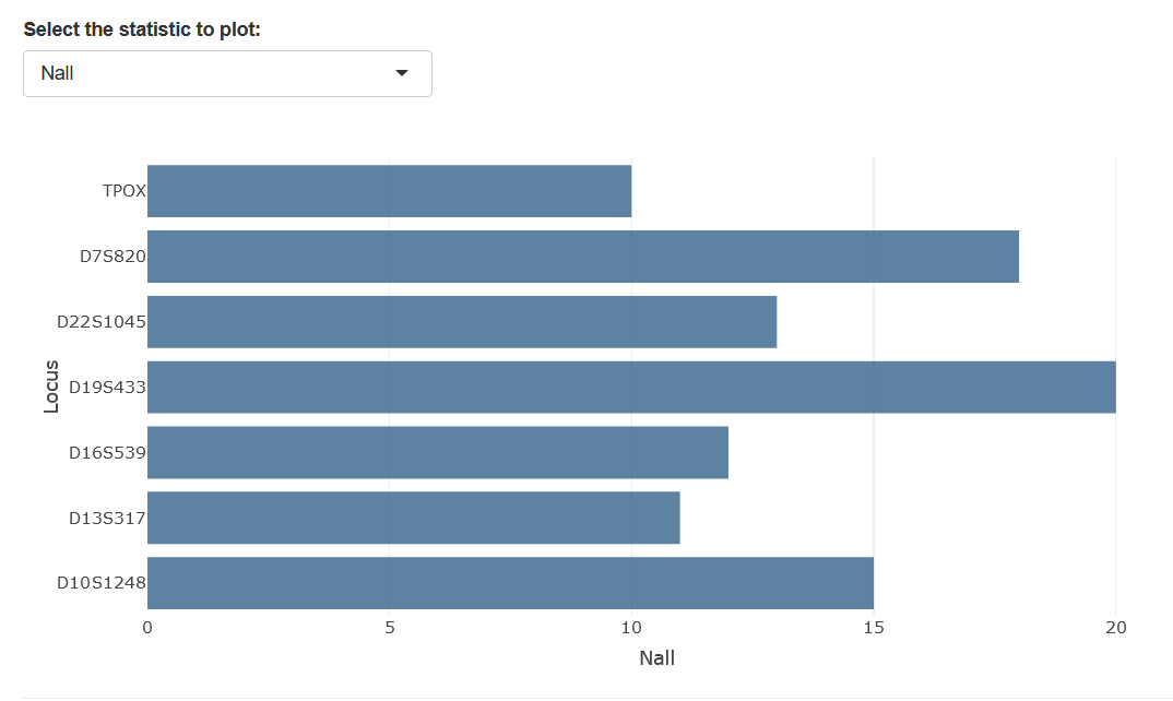
Below the forensic parameters table, You can select the metric you would like to represent using the drop-down menu.
3.2 Details on the forensic parameters
3.2.1 Random match probability (PM)
The Random match probability, or probability of matching (PM), is defined as the probability of observing a random match between two unrelated individuals.
Formula
\[ PM = \sum_i (G_i)^2, \] where \(G_i\) is the frequency of the genotype \(i\) at a given locus in the population.
Interpretation
Computing \(PM\) means calculating, for a given locus, the frequency of each genotypes. Then we take the square of each frequency, i.e. we multiply it by itself. Finally, we sum the values of each genotype.
The intuition behind it is that if we observe a random match in a population when looking at a single locus, it means that our two samples have the same genotype at that locus. In terms of probabilities, sampling a specific genotype in the population has a probability equal to its frequency. And sampling the same genotype a second time (i.e., observing a match), is the probability of sampling this genotype multiplied by itself.
As an example, say the genotype “12-14” has a frequency of 5% in the population, the probability of having a random match between two individuals having the same genotype is 0.05 x 0.05.
To get an overall probability of matching, we sum this over all possible genotypes in our population.
References
Butler (2014) - Advanced Topics in Forensic DNA Typing: Interpretation, pp. 264-265. Academic Press.
Jones (1972). Blood samples: probability of discrimination. Journal of the Forensic science Society, 12(2), 355-359.
Sensabaugh (1982) - Isozymes in forensic science. In: Isozymes Current Topics in Biological and Medical Research Volume 6 (editor, Liss, A. R.) pp. 247–282.
3.2.2 Power of Discrimination (PD)
The power of discrimination (PD) is defined as the probability of discriminating between two unrelated individuals.
Formula
\[ PD = 1 - PM \]
Interpretation
PD is simply 1 - PM. Instead of looking at the probability of matching, we are interested in the probability of “not matching”, i.e. the probability of discrimination.
Reference
Butler (2014) - Advanced Topics in Forensic DNA Typing: Interpretation, pp. 264-265. Academic Press.
3.2.3 Gene diversity
Gene diversity (\(GD\), sometimes simply \(D\)), also called expected heterozygosity (\(H_{\mathrm{exp}}\)), is computed using the following estimator:
Formula
\[ H_{\mathrm{exp}} = GD = \frac{n}{n - 1} \left( 1 - \sum_{i=1}^{n}(p_i)^2 \right), \]
where \(n\) is the number of gene copies sampled (i.e., the sample size for haploid samples, and twice the sample size for diploid samples) and \(p_i\) is the frequency of the \(i^{th}\) allele in the population.
NB: This statistic is sometimes called expected heterozygosity as it has first been developed to study diploid organisms. As this metric is a quantification of genetic diversity and can also be computed for haploid samples, gene diversity (GD) is a more generic term.
Interpretation
It is the probability that an individual will be heterozygous at a given locus.
As an example, a value of \(GD\) of 0.6 means that there is a 60% chance of being heterozygote at this locus.
It depends directly on the genetic diversity at this locus, which itself depends on allele frequencies in your population.
Say we have two alleles in a given population, genetic diversity will be higher in a population with allele frequencies 0.5 and 0.5 than in a population where frequencies are 0.1 and 0.9 (as less heterozygotes can be made with rare alleles). This rationale can be extended to any number of alleles.
References
Butler (2014) - Advanced Topics in Forensic DNA Typing: Interpretation, pp. 264-265. Academic Press.
Nei (1973). Analysis of gene diversity in subdivided populations. Proc. Natl. Acad. Sci. USA 70: 3321–3323.
3.2.4 Polymorphism Information Content (PIC)
Formula
The Polymorphism Information Content (PIC) is computed as follow:
\[ PIC = 1 - \sum_{i=1}^{n} p_i^2 - \sum_{i=1}^{n-1} \sum_{j=i+1}^{n} 2p_i^2p_j^2, \] where \(p_i\) and \(p_j\) are allele frequencies.
Interpretation
The PIC can be interpreted as:
the probability that the maternal and paternal alleles of a child are deducible
or, the probability of being able to deduce which allele a parent has transmitted to the child.
References
Botstein, White, Skolnick, Davis (1980). Construction of a genetic linkage map in man using restriction fragment length polymorphisms. American journal of human genetics, 32(3), 314.
Butler (2014) - Advanced Topics in Forensic DNA Typing: Interpretation, pp. 264-265. Academic Press.
3.2.5 Power of Exclusion (PE)
Formula
The power of exclusion (\(PE\)) is defined as:
\[ PE = h^2\left(1 - 2hH^2\right), \]
where \(h\) is the proportion of heterozygous individuals and \(H\) the proportion of homozygous individuals in the population sample.
Interpretation
The power of exclusion depends on the observed proportions of heterozygous and homozygous individuals in a population. These proportions, multiplied as in the equation above, give the mean exclusion probability for a paternity test. Intuitively, the more diverse the population is, the greater this value is, as diversity is related to heterozygosity (see above).
References
Butler (2014) - Advanced Topics in Forensic DNA Typing: Interpretation, pp. 264-265. Academic Press.
Fisher (1951) - Standard Calculations for Evaluating a Blood-Group System. Heredity, 5: 95-102.
3.2.6 Typical Paternity Index (TPI)
Finally, the typical paternity index (\(TPI\)) reflects the “mean PI for random non-excluded men“ in trio cases (father-mother-child) for a given locus.
Formula
Let \(H\) be the frequency of homozygotes, then
\[ TPI = \frac{1}{2H} \]
Interpretation
Unlike the other parameters, the typical paternity index values are not in the 0-1 range and cannot be interpreted as a probability. It is a ratio of 1 divided by twice the frequency of homozygotes in the population. This is an odds ratio, measuring how many times more likely that a possible father is the actual father than a randomly selected man in the population, on average (typical case).
Reference
Butler (2014) - Advanced Topics in Forensic DNA Typing: Interpretation, pp. 264-265. Academic Press.